This blog explains how to build a Student Performance Classifier with Azure Machine Learning. This classifier predicts if a student will pass or fail Mathematics. The complete experiment can be downloaded from the Azure Machine Learning Gallery.
Description of the Student Performance Classifier
This classifier predicts a student’s performance for Mathematics (fail or pass). It is based on the Student Performance Data Set. This data set contains information about student achievement in secondary education of two Portuguese schools. The data attributes include student grades, demographic, social and school related features and it was collected by using school reports and questionnaires. Two datasets are provided regarding the performance in two distinct subjects: Mathematics (mat) and Portuguese language (por). In the paper of Cortez and Silva (2008), the two datasets were modeled under binary/five-level classification and regression tasks. For this experiment, we will focus only on the binary classification.
In their conclusion, Cortez and Silva recommend to use a student prediction engine as part of a school management support system. Besides, they encourage the exploration of automatic feature selection. Azure Machine Learning offers the possibility to offer prediction models as a service, which could address the first recommendation. Secondly, it offers the Filter Based Feature Selection module.
Data Processing and Analysis
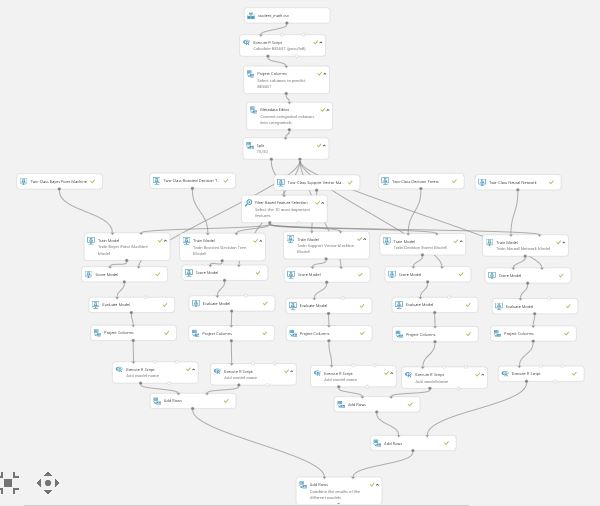
This experiment will test several binary classification models (Two-Class Boosted Decision Tree, Two-Class Support Vector Machine, Two-Class Decision Forest, Two-Class Neural Network, and Two-Class Bayes Point Machine). The results will be compared using an Execute R module.
In this sample we use the Student Performance Data from its source: http://archive.ics.uci.edu/ml/datasets/Student+Performance. More info can also be found on the UCI repository. We wil use only the Mathematics data set, which we uploaded to the Azure Machine Learning environment.
The data has been collected using school report and questionnaires. This resulted in a dataset with 350 rows and 33 columns.
- 1 school – student’s school (binary: ‘GP’ – Gabriel Pereira or ‘MS’ – Mousinho da Silveira)
- 2 sex – student’s sex (binary: ‘F’ – female or ‘M’ – male)
- 3 age – student’s age (numeric: from 15 to 22)
- 4 address – student’s home address type (binary: ‘U’ – urban or ‘R’ – rural)
- 5 famsize – family size (binary: ‘LE3’ – less or equal to 3 or ‘GT3’ – greater than 3)
- 6 Pstatus – parent’s cohabitation status (binary: ‘T’ – living together or ‘A’ – apart)
- 7 Medu – mother’s education (numeric: 0 – none, 1 – primary education (4th grade), 2 5th to 9th grade, 3 secondary education or 4 higher education)
- 8 Fedu – father’s education (numeric: 0 – none, 1 – primary education (4th grade), 2 5th to 9th grade, 3 secondary education or 4 â higher education)
- 9 Mjob – mother’s job (nominal: ‘teacher’, ‘health’ care related, civil ‘services’ (e.g. administrative or police), ‘at_home’ or ‘other’)
- 10 Fjob – father’s job (nominal: ‘teacher’, ‘health’ care related, civil ‘services’ (e.g. administrative or police), ‘at_home’ or ‘other’)
- 11 reason – reason to choose this school (nominal: close to ‘home’, school ‘reputation’, ‘course’ preference or ‘other’)
- 12 guardian – student’s guardian (nominal: ‘mother’, ‘father’ or ‘other’)
13 traveltime – home to school travel time (numeric: 1 – <15 min., 2 – 15 to 30 min., 3 – 30 min. to 1 hour, or 4 – >1 hour) - 14 studytime – weekly study time (numeric: 1 – <2 hours, 2 – 2 to 5 hours, 3 – 5 to 10 hours, or 4 – >10 hours)
- 15 failures – number of past class failures (numeric: n if 1<=n<3, else 4)
- 16 schoolsup – extra educational support (binary: yes or no)
- 17 famsup – family educational support (binary: yes or no)
- 18 paid – extra paid classes within the course subject (Math or Portuguese) (binary: yes or no)
- 19 activities – extra-curricular activities (binary: yes or no)
- 20 nursery – attended nursery school (binary: yes or no)
- 21 higher – wants to take higher education (binary: yes or no)
- 22 internet – Internet access at home (binary: yes or no)
- 23 romantic – with a romantic relationship (binary: yes or no)
- 24 famrel – quality of family relationships (numeric: from 1 – very bad to 5 – excellent)
- 25 freetime – free time after school (numeric: from 1 – very low to 5 – very high)
- 26 goout – going out with friends (numeric: from 1 – very low to 5 – very high)
- 27 Dalc – workday alcohol consumption (numeric: from 1 – very low to 5 – very high)
- 28 Walc – weekend alcohol consumption (numeric: from 1 – very low to 5 – very high)
- 29 health – current health status (numeric: from 1 – very bad to 5 – very good)
- 30 absences – number of school absences (numeric: from 0 to 93)
- 31 G1 – first period grade related to the course subject (numeric: from 0 to 20)
- 31 G2 – second period grade related to the course subject (numeric: from 0 to 20)
- 32 G3 – final grade related to the course subject (numeric: from 0 to 20, output target)
The following diagram shows the entire experiment (as the experiment is too big to fit on the screen, it would be better to download the sample and view it in Azure ML studio):
First, we use the module Execute R Script to apply some basic tranformations. We removed the observations with G3 score 0. We follow the steps from the paper and create new variables for the nominal variables.
# Map 1-based optional input ports to variables
data <- maml.mapInputPort(1) # class: data.frame
# delete observations with score 0
data <- subset(data, data$G3>=1)
# create vectors for categorical, multi-categorical and numeric data
cat_data <- c(“school”,”sex”,”address”,”famsize”,”Pstatus”,”schoolsup”,”famsup”,
“paid”,”activities”, “nursery”,”higher”, “internet”,”romantic”)
multi_cat <- c(“Mjob”,”Fjob”,”reason”,”guardian”)
numeric_data <- c(“age”,”Medu”,”Fedu”,”traveltime”,”studytime”,
“famrel”,”freetime”,”goout”,”Dalc”,”Walc”,”health”,”absences”,
“failures”,”G2″,”G1″,”G3″)
# transform multi categoricals
for(i in multi_cat) {
for(level in unique(data[,i])){
data[paste(paste(“bin”,i,sep=”_”), level, sep = “_”)] <- ifelse(data[,i] == level, “yes”, “no”)
}
}
# select dummy variables
new_multi_cat <- grep(“bin_”,colnames(data))
new_multi_cat <- names(data)[new_multi_cat]
# make them factors
for (i in new_multi_cat) {
data[,i] <- as.factor(data[,i])
}
# create a new dataset based on prior categorical, new binary, and numeric data
select <- c(cat_data, new_multi_cat, numeric_data)
data <- data[,select]
# calculate pass/fail
data$result <- as.factor(sapply(data$G3,function(res)
if (res >=10) ‘pass’ else ‘fail’))
# Select data.frame to be sent to the output Dataset port
maml.mapOutputPort(“data”);
We added an instance of the Project Columns module to exclude the original end score variable (G3). Thereafter, we use the Metadata Editor module specify all the non-numeric columns to be a categorical variable.
We Split the dataset in a training (70%) and a test (30%) set.
To select the most important predictors, we use the Filter Based Feature Selection module, selecting the 10 most important features. This results in the selection of G2, G11, failures, absences, goout, schoolsup, studytime, Fedu, age, Mjob (other) as the most important features related to the final result.
To find the best-fitting model, we will test 5 different models: Two-Class Boosted Decision Tree, Two-Class Support Vector Machine, Two-Class Decision Forest, Two-Class Neural Network, and Two-Class Bayes Point Machine. This selection has been based on the chosen models in the original paper.
Results
We compared the results, using an Execute R module to combine the results. The Bayes Point Machine, Support Vector Machine, and Decision Forest models gave very similar results, but when it comes to precision, the Decision Forest model was the most precise.
| Model | Accuracy | Precision | Recall | F-Score | AUC | Average Log Loss | Training Log Loss |
| Bayes Point Machine | 0.93 | 0.94 | 0.97 | 0.95 | 0.98 | 0.22 | 63.82 |
| Boosted Decision Tree | 0.91 | 0.93 | 0.93 | 0.93 | 0.97 | 0.22 | 63.60 |
| Support Vector Machine | 0.93 | 0.96 | 0.93 | 0.95 | 0.98 | 0.16 | 74.38 |
| Decision Forest | 0.93 | 0.99 | 0.92 | 0.95 | 0.98 | 0.16 | 72.99 |
| Neural Network | 0.89 | 0.94 | 0.89 | 0.92 | 0.97 | 0.22 | 63.54 |
Sources
Data
dataset: http://archive.ics.uci.edu/ml/datasets/Student+Performance
Paper
P. Cortez and A. Silva. Using Data Mining to Predict Secondary School Student Performance. In A. Brito and J. Teixeira Eds., Proceedings of 5th FUture BUsiness TEChnology Conference (FUBUTEC 2008) pp. 5-12, Porto, Portugal, April, 2008, EUROSIS, ISBN 978-9077381-39-7.
Available at: [Web Link]


